Configuration

Configuring the anonymization process

In the configuration perspective, data can be imported and transformation rules, privacy models and utility measures can be selected and parameterized.

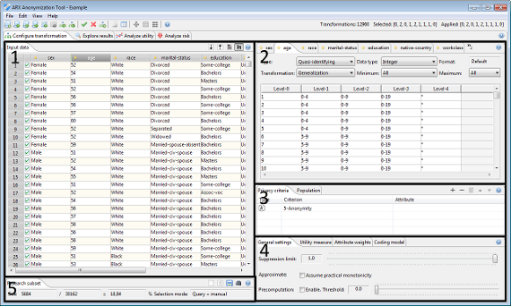
The perspective is divided into five main areas.

Area 1 shows the current input dataset:

• The table displays further information on specified attribute metadata.

Area 2 provides a means to specify attribute metadata and view generalization hierarchies:

• Attribute types and data types can be specified.
• Generalization hierarchies can be modified.

Area 3 supports the configuration of privacy models:

• Multiple privacy models can be selected and configured. Further parameters can be specified in dedicated tabs.

Area 4 supports the configuration of utility measures:

• A single utility measure can be configured and selected as an objective function.

Area 5 provides methods for extracting a research sample:

• With this concept ARX supports the specification of population tables, by defining the dataset which is to be anonymized as a sample of the dataset that has been loaded.
• The sample can be selected manually, drawn randomly, or selected by query or by matching with another dataset.

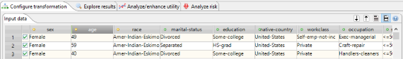
Tables representing input and output data

ARX displays input and output data in special tables with headers which indicate attribute types by different colors:

Each record is further associated with a checkbox. These checkboxes indicate, which records are contained in the specified research sample. The checkboxes in the view for output datasets, indicate the sample that was specified when the anonymization process was last executed. They cannot be edited. The checkboxes in the view for the input dataset represent the current research sample. They are editable.

Each table offers a few options that are accessible via buttons in the top-right corner:

1. The first button sorts the data according to the currently selected column.
2. The second button sorts the output dataset according to all quasi-identifiers and then highlights equivalence classes.
3. The third button controls whether all records are shown or only records contained in the research sample.

Specifying attribute properties

Attribute properties can be set in the tabs "data transformation" and "attribute metadata" within this perspective. To set an attribute's properties, it must first be selected in the tabular view of the dataset. The views in the tabs will be linked with the selected attribute and updated accordingly.

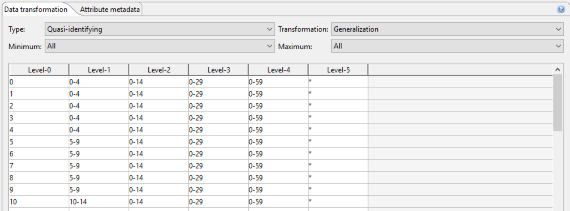
Data transformation

The transformation tab can be used to set the type of an attribute and the associated transformation method. The transformation tab also displays the attribute's generalization hierarchy and provides a context menu for in-place editing.

Supported attribute types:

1. Identifying attributes will be removed from the dataset.
2. Quasi-identifying attributes will be transformed.
3. Sensitive attributes will be kept as-is but they can be protected using privacy models, such as t-closeness or l-diversity.
4. Insensitive attributes will be kept unmodified.

Note: the specified type of an attribute is also indicated by a color coded bullet, next to the attribute name, in the input tab.

Note: since version 3.7.0 there are also specific buttons that can be used to assign a certain attribute type to all attributes in the dataset.

Supported transformation methods include generalization, microaggregation and suppression. When generalization is selected, minimum and maximum generalization levels can be specified. Microaggregation may be performed with or without prior clustering using the specified value generalization hierarchies, Moreover, the aggregation function and how missing values should be handled can be specified.

The associated value generalization hierarchy is displayed in tabular form. Original attribute values are displayed in the leftmost column, with generalization levels increasing from left to right. Right clicking the table brings up a context menu providing access to editing functionalities. This can be used to create simple hierarchies or to simple modifications to existing hierarchies. Moreover, hierarchies representing attribute suppression can be created. For creating more complex hierarchies, ARX supports several wizards, which can be launched from the application menu and the tool bar.

Attribute metadata

This view can be used to specify data types (including formats) of attributes. Please note that the correct data type is needed to use most of the wizards for hierarchy creation.

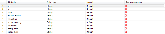
Supported data types:

1. String: a generic sequence of characters. This is the default data type.
2. Integer: a data type for numbers without a fractional component.
3. Decimal: a data type for numbers with fractional component.
4. Date/time: a data type for dates (with or without time).
5. Ordinal: string variables with an ordinal scale.

Data types can be set by right clicking on an attribute's row in the table. When needed, ARX will ask for a suitable format string. Specifying a data type is optional but yields better results when creating generalization hierarchies and visualizing data in the analysis perspective.

Variables can be defined as "response variables" in modeling efforts that will be performed using output data. When combined with an appropriate data quality model, ARX will then try to minimize impacts on the structural relationships between quasi-identifying variables and the specified response variables.

Information on supported decimal formats can be found here.

Information on supported date formats can be found here.

Creating generalization hierarchies

ARX offers different methods for creating generalization hierarchies for different types of attributes. Generalization hierarchies created with the wizard are stored as functions, meaning that they can be created for the entire domain of an attribute without explicitly addressing the specific values in a concrete dataset. This enables the handling of continuous variables. Moreover, hierarchy specifications can be imported and exported and they can thus be reused for anonymizing different datasets with similar attributes. It is important that adequate data types are specified prior to using the wizard. The wizard can be used to create four different types of hierarchies:

1. Masking-based hierarchies: this general-purpose mechanism allows creating hierarchies for a broad spectrum of attributes.
2. Interval-based hierarchies: these hierarchies can be used for variables with a ratio scale.
3. Order-based hierarchies: this method can be used for variables with an ordinal scale.
4. Date-based hierarchies: this method can be used for dates.

Masking-based hierarchies

Masking is a flexible mechanism that can be applied to many types of attributes and which is especially suitable for alphanumeric codes, such as ZIP codes. The following image shows a screenshot of the respective wizard:

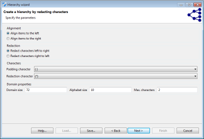
In the wizard, masking follows a two-step process. First, values are aligned either to the left or to the right. Then the characters are masked, again, either from left to right, or from right to left. All values are adjusted to a common length by adding padding characters. This character, as well as the character used for masking can be specified by the user.

Interval-based hierarchies

Intervals are a natural means of generalization for values with a ratio scale, such as integers or decimals. ARX offers a graphical editor for efficiently defining sets of intervals over the complete range of variables having any of the above data types. First a sequence of intervals can be defined on the left side of the view. In the next step, subsequent levels consisting of groups of intervals from the previous level can be specified. Each group combines a given number of elements from the previous level. Any sequence of intervals or groups is automatically repeated to cover the complete range of the attribute. For example, to generalize arbitrary integers into intervals of length 10, only one interval [0, 10] needs to be defined. Defining a group of size two on the next level, automatically generalizes integers into groups of size 20. As is shown in the image (W1), the editor visually indicates automatically created repetitions of intervals and groups.

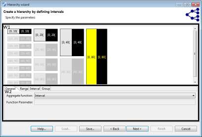
To be able to create labels for intervals, each element must be associated with an aggregate function (W2). The following aggregate functions are supported:

1. Set: a set-representation of input values is returned.
2. Prefix: a set of prefixes of the input values is returned. A parameter allows defining the length of these prefixes.
3. Common-prefix: returns the largest common prefix.
4. Bounds: returns the first and last elements of the set.
5. Interval: an interval between the minimal and maximal value is returned.
6. Constant: returns a predefined-constant value.

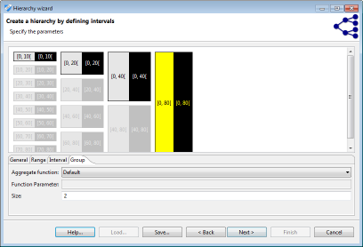
Clicking on an interval or a group prompts an editor which can be used for specifying parameters. Elements can be removed, added and merged by right-clicking their graphical representation. Intervals are defined by a minimum (inclusive) and maximum (exclusive) bound. Groups are defined by their size:

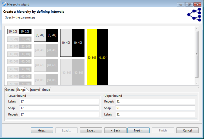
Interval-based hierarchies might define ranges in which they are to be applied. Any value out of the range defined by "minimum value" or "maximum value" will produce an error message. This can be used to implement sanity checks. Any value between the minimal or maximal value and the "bottom coding" or "top coding" values will be top- or bottom-coded. If values fall into an interval stretching from the bottom coding or top coding limit to the "snap" limit, it will be extended to the bottom or top coding limit. Within the remaining range intervals will be repeated..

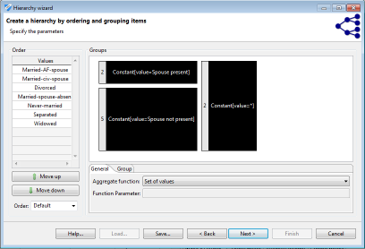
Order-based hierarchies

Order-based hierarchies follow a similar principle as interval-based hierarchies, but they can be applied to attributes with ordinal scale. In addition to the types of attributes covered by interval-based hierarchies this includes strings, using their lexicographical order, and ordinals. First, attributes within the domain are ordered as defined by the user or the data type. Second, ordered values can be grouped using a mechanism similar to the one used for interval-based hierarchies. Note that order-based hierarchies are especially useful for ordinal strings and therefore display the complete domain of an attribute instead of only the values contained in the concrete dataset. The mechanism can be used to create semantic hierarchies from a pre-defined meaningful ordering of the domain of a discrete variable. Subsequent generalizations of values from the domain can be labeled with user defined constants.

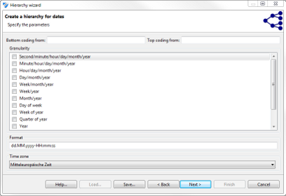
Date-based hierarchies

This wizard supports the creation of hierarchies for dates by specifying the granularity of output data at increasing generalization levels. Please note that it is important to specify granularity levels that form an hierarchy (e.g. day-of-week can typically not be followed by week-of-year, because the same day-of-week can be generalized to different weeks of a year). When this constraint is violated, ARX will raise an error message during the anonymization process.

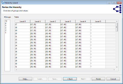
In a final step, all wizards show a tabular representation of the resulting hierarchy for the current input dataset. Additionally, the number of groups on each level is calculated. The functional representation created in the process can be exported and reused for different datasets with similar attributes.

Privacy models, population properties, costs and benefits of data sharing

Privacy models can be selected and configured in the following view:

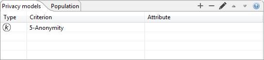
Models that have been selected are shown in the table. Privacy models can be added or removed by clicking the plus or minus button, respectively. The third button brings up a dialog for parameterization.

Most buttons will bring up the following configuration dialog. Here, the arrow pointing downwards can be used to select a parameterization out of a set of presets for the selected privacy model.

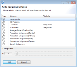
k-Anonymity, k-Map, δ-presence, risk-based privacy models, differential privacy and the game-theoretic model focus on quasi-identifiers and they can therefore always be enabled. In contrast, l-diversity, t-closeness, β-likeness and δ-disclosure privacy focus on sensitive attributes. They can thus only be enabled if a sensitive attribute has been selected. Some models further require particular settings (e.g. a value generalization hierarchy must be specified to be able to use t-closeness with hierarchical ground distance. Some privacy models (e.g. k-map and δ-presence) require a population table, which is supported in ARX by defining the dataset which is to be anonymized as a (research) sample of the dataset which has been loaded.

Note: If a model based on population uniqueness is used, properties of the underlying population must also be specified. This is supported by the following section of the perspective:

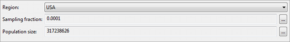
Note: Models based on population uniqueness assume that the dataset is a uniform sample of the population. If this is not the case, results may be inaccurate.

Note: The game-theoretic model is based on a cost/benefit analysis and therefore requires the specification of various parameters which can be found in an associated section of the perspective:

Here, the following parameters must be specified:

1. Adversary cost: the amount of money needed by an attacker for trying to re-identify a single record.
2. Adversary gain: the amount of money earned by an attacker for successfully re-identifying a single record.
3. Publisher benefit: the amount of money earned by the data publisher for publishing a single record.
4. Publisher loss: the amount of money lost by the data publisher, e.g. due to a fine, if a single record is attacked successfully.

Transformation and utility model

In the first tab of this view, general properties of the transformation process can be specified.

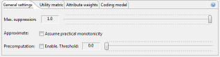
The first slider allows to define the suppression limit, which is the maximal number of records that can be removed from the input dataset. The recommended value for this parameter is "100%". The option "Approximate" can be enabled to compute an approximate solution with potentially significantly reduce execution times. The solution is guaranteed to fulfill the given privacy settings, but it might not be optimal regarding the data utility model specified. The recommended setting is "off". For some utility measures, precomputation steps can be used, which may also significantly reduced execution times. Precomputation is switched on when, for each quasi-identifier, the number of distinct data values divided by the total number of records in the dataset is lower than the configured threshold. Experiments have shown that 0.3 is often a good value for this parameter. The recommended setting is "off".

The second tab allows specifying the model for quantifying data quality which will be used as an optimization function during the anonymization process.

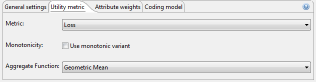
ARX will use the specified model to assign "scores" to potential solution candidates. A lower score is associated with higher data quality, less loss of information, higher publisher payout or increased classification accuracy, depending on the selected model. Note, however, that scores may significantly deviate from the actual values that would be returned by the models due to internal optimizations in ARX. As a consequence, you should never report "scores" as a measure describing data quality. To obtain such measures, the utility analysis perspective should be used.

Monotonicity is a property of privacy and utility models that can be exploited to make the anonymization process more efficient. In real-world settings, however, models are almost never monotonic due to the complexity of the transformation methods used by the software. ARX can be configured to always assume monotonicity, which will speed-up the anonymization process significantly but which may also lead to significant reductions in output data quality. The recommended setting is "off". ARX also supports user-defined aggregate functions for many quality models. These aggregate functions will be used to compile the estimates obtained for the individual attributes of a dataset into a global value. The recommended setting is "Arithmetic mean".

Most models support weights that can be assigned to attributes to specify their importance using the following view:

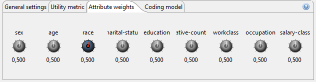
Each of the knobs can be used to associate a weight to a specific quasi-identifier. When anonymizing the dataset, ARX will try to reduce the loss of information for attributes with higher weights.

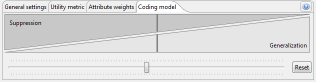
Some quality models also support specifying whether generalization or suppression should be preferred when transforming data:

Defining a research sample

In this view, a research sample can be specified. It represents a sample of the overall dataset that will be anonymized and exported. This feature can be used to anonymize data using a population table. Privacy models that can consider this information include δ-presence, k-map and the game-theoretic approach. It is also considered by some methods for risk analysis. The buttons in the top-right corner provide access to different options for extracting a sample from the dataset:

1. Selecting no records.
2. Selecting all records.
3. Selecting records by matching the current dataset against an external dataset.
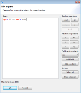
4. Selecting records by querying the dataset.
5. Selecting records by random sampling.

The view will show the size of the current sample and the method with which it was created. At any time, the research sample can be altered by clicking the checkboxes shown in the data tables. The query syntax is as follows: fields and constants must be enclosed in single quotes. In the example 'age' is a field and '50' is a constant. The following operators are supported: >, >=, <, <=, =, or, and, ( and ). The dialog dynamically shows the number of rows matching the query and displays error messages in case of syntactic errors.

Project settings

The settings window is accessible from either the application menu or the application toolbar.

The Project section can be used to alter general project properties:

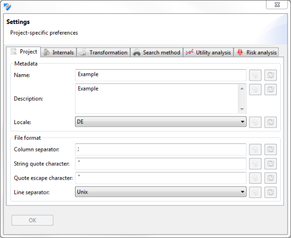
• Project meta data, including name, description and localization.
• The syntax for CSV import and export.

The Internals section can be used to adjust performance and visualization parameters:

• Snapshot settings control the space-time trade-off during data anonymization. Larger (relative) snapshot sizes will typically reduce execution time but increase memory consumption.
• Some analyses and visualizations can be disabled when very large datasets are handled.

The Transformation section provides options for altering and simplifying the presentation of transformed data:

• Record suppression can enabled or disabled for non-anonymous output data.
• Attribute suppression can be enabled or disabled for sensitive and insensitive attributes.

The Search method section can be used to configure the search strategy and risk based anonymization:

• An heuristic search using a time limit can be enabled for high-dimensional data.
• Utility-driven record suppression can be disabled to improve execution times.

The Utility analysis section can be used to refine summary statistics and quality measurements:

• Summary statistics may be calculated with or without list-wise deletion.
• The use of functional hierarchies during the anonymization process can be disabled.
• Parameters impacting the performance of the analysis of the usefulness of output data for classification tasks may be altered.

The Risk analysis section provides configuration options for the integrated solver for non-linear equation systems:

• Optimization parameters include the total number of iterations, iterations per try and the required accuracy.

Performing the anonymization

ARX provides a dedicated dialog for selecting an adequate search strategy, configuring aspects of the transformation model, and, finally, starting the anonymization process:

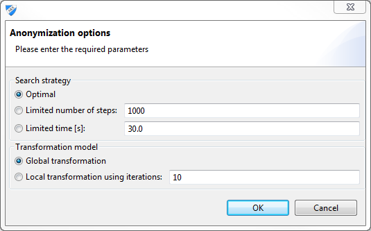
Three different search strategies are available:

1. Optimal search strategy.
2. Heuristic search strategy terminating after a pre-defined number of search steps.
3. Heuristic search strategy terminating after a pre-defined amount of time.

Please note that the optimal search strategy reliably determines the transformation resulting in the highest possible quality of output data but scalability issues may occur when processing large datasets. The heuristic search strategies are often able to determine the optimal strategy very quickly, but optimality can not be guaranteed. For large datasets they work on a best-effort basis.

Two different transformation models are supported:

1. Global transformation: the same transformation strategy will be applied to all records in the dataset.
2. Local transformation: different transformation strategies can be applied to different subset of the records in the dataset. A limit on the number of different transformations that may be used can be specified.

By combining the different transformation models with different transformation rules for the individual attributes a wide variety of transformation methods can be used in combination:

• The global transformation can be used to implement (1) full-domain generalization, (2) top- and bottom-coding (there is a shortcut for creating according rules in the hierarchy editor), (3) attribute-suppression (there is a shortcut for creating according rules in the hierarchy editor), (4) record-suppression and (5) micro-aggregation.
• The local transformation can be used to implement (1) full-domain generalization (by defining a fixed generalization level), (2) top- and bottom-coding (by defining a fixed generalization level), (3) local generalization, (4) attribute-suppression (by defining a fixed generalization level), (5) cell-suppression and (6) micro-aggregation.
• In addition, random sampling can be performed in the respective view in the configuration perspective.

While it is not generally true that global transformation will involve less computational costs than local transformation, the former is typically faster. In each iteration of the local transformation method the selected search strategy will be used. Note, however, that using the optimal strategy in each iteration does not necessarily imply that overall solution computed through local transformation will also be optimal.