Utility analysis

Analyzing data utility

This perspective can be used to analyze the quality and utility of output data for the anticipated usage scenario. For this purpose, it is possible to compare the transformed dataset to the original input dataset. In the upper part, this perspective will display the original data (area 1) and the result of the currently selected transformation (area 2). Both tables are synchronized when they are browsed using the horizontal or vertical scroll bars. The areas 3 and 4 allow to compare statistical information about the currently selected attribute(s).

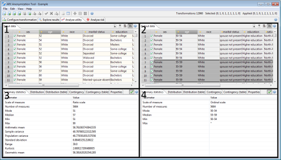
The view further displays results of univariate and bivariate statistics and basic properties about the input and output dataset. Moreover, it provides access to statistics about the distribution of equivalence classes and suppressed records. Finally, the suitability of output data as a training set for building classification models can be analyzed.

Note: ARX tries to present comparable data visualizations for original and transformed datasets. For this purpose, it uses information from the attributes' data types and relationships between values extracted from the generalization hierarchies. As a result, specifying reasonable data types and hierarchies will increase the quality and usefulness of data visualizations.

Comparing input and output data

In this section a transformed dataset can be compared to the original input dataset. The horizontal and vertical scrollbars of both tables are synchronized.

The checkboxes indicate, which rows are part of the research sample. The checkboxes in the table displaying the output dataset indicate the sample that was selected when the anonymization process was performed. They cannot be altered. The checkboxes in the table displaying the input dataset represent the current research sample. They are editable.

Each table offers a few options, which are accessible via buttons in the top-right corner of the view:

1. Pressing the first button will sort the data according to the currently selected attribute.
2. Pressing the second button will sort the output dataset according to all quasi-identifiers and then highlight the equivalence classes.
3. Pressing the third button will toggle whether all records of the dataset are displayed or only records that are part of the research sample.

Summary statistics

The first tab on the bottom of the utility analysis perspective shows summary statistics for the currently selected attribute.

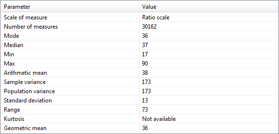
The displayed parameters depend on the scale of measure of the variable. For attributes with a nominal scale, the following parameters will be provided:

• Mode.

For attributes with an ordinal scale, the following additional parameters will be displayed:

• Median, minimum, maximum.

For attributes with an interval scale, the following additional parameters will be provided:

• Arithmetic mean, sample variance, population variance, standard deviation, range, kurtosis.

For attributes with a ratio scale, the following additional parameters will be displayed:

• Geometric mean.

Note: These statistical parameters are calculated using list-wise deletion, which is a method for handling missing data. With this method, an entire record is excluded from analysis if any single value is missing. This behavior can be changed in the project settings.

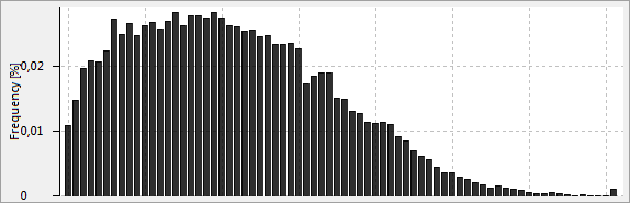
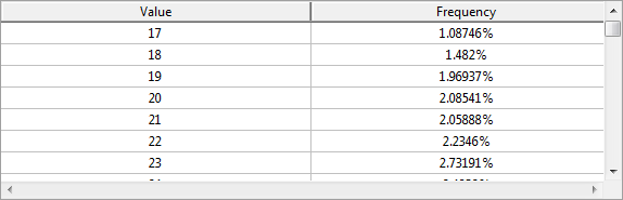
Empirical distribution

This view shows a histogram or a table visualizing the frequency distribution of the values of the currently selected attribute.

From Wikipedia: In statistics, a frequency distribution is a table that displays the frequency of various outcomes in a sample. Each entry in the table contains the frequency or count of the occurrences of values within a particular group or interval, and in this way, the table summarizes the distribution of values in the sample.

From Wikipedia: A histogram is a graphical representation of the distribution of numerical data. It is an estimate of the probability distribution of a continuous variable. To construct a histogram, the first step is to "bin" the range of values - that is, divide the entire range of values into a series of intervals - and then count how many values fall into each interval.

Note: ARX tries to present comparable data visualizations of properties of the original and transformed data sets. For this purpose, it uses information from the attributes' data types and relationships between its values, which are extracted from the generalization hierarchies. As a consequence, specifying reasonable data types and hierarchies will increase the quality and comparability of data visualizations.

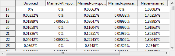
Contingency

This view shows a heat map or a table visualizing the contingency of two selected attributes.

Contingency refers to the multivariate frequency distribution of the variables.

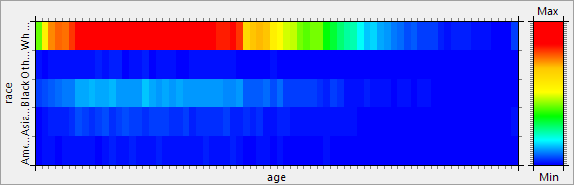
Note: ARX tries to present comparable data visualizations of properties of the original and transformed datasets. For this purpose, it uses information from the attributes' data types and relationships between its values, which are extracted from the generalization hierarchies. As a consequence, specifying reasonable data types and hierarchies will increase the quality and usefulness of data visualizations.

Equivalence classes and records

This view summarizes information about the records in the dataset. It shows the minimal, maximal and average size of the equivalence classes, the number of classes as well as the number of suppressed and remaining records.

Note, that an "equivalence class" describes a set of records which are indistinguishable regarding the specified quasi-identifying variables. Sometimes, equivalence classes are also called "cells".

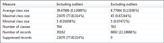
For the output dataset, all parameters are calculated in two variants. One variant considers suppressed records and the other variant ignores suppressed records.

Note: The variant that ignores suppressed records uses list-wise deletion, which is a method for handling missing data. In this method, an entire record is excluded from the analysis if any single value is missing.

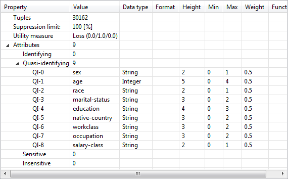
Properties of input data

This view displays basic properties about the input dataset and the configuration used for anonymization. These properties include the number of records and the suppression limit as well as a shallow specification of all attributes in the dataset, including data about the associated transformation methods.

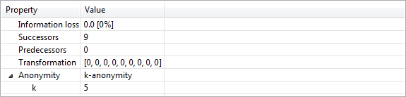
Properties of output data

This view displays basic properties about the selected data transformation as well as the resulting output dataset. These properties include the score calculated using the specified utility measure and further settings (e.g. attribute weights), the number of suppressed records, the number of equivalence classes and the number of classes containing suppressed records. If the transformation is privacy-preserving, a complete specification of all privacy models is provided.

Note: The information provided in this view is based on the specification which has been defined in the configuration perspective prior to performing the anonymization process. The state of the workbench will remain unchanged, even if these definitions are changed. To bring changes into effect, the data anonymization process needs to be executed again.

Classification performance

This view can be used to configure classification models and their parameters as well as to compare the performance of these models trained on input and anonymized output data. Please note that ARX supports a specific quality model for optimizing output data towards suitability as a training set for model generation.

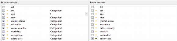
In the view displayed at the bottom left, feature and target variables can be selected and feature scaling functions may be specified:

In the view displayed at the bottom right different types of classification models can be selected and configured:

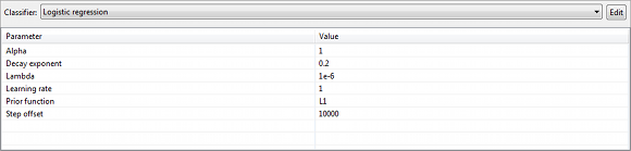
ARX currently supports the following types of classification models:

1. Logistic regression
2. Random forest
3. Naive Bayes

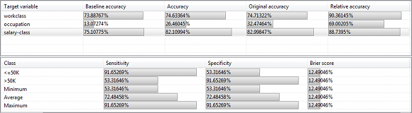
At the top, two different views can be selected by tabs ("Overview" and "ROC curves"). For input as well as output data, these views show different results of the performance analysis. Performance measures are typically expressed relative to the performance of a trivial ZeroR classifier trained on unmodified input data and the selected type of model also trained on input data. Results are obtained using k-fold cross-validation.

The tables in the view "Overview" display (relative) classification accuracies as well as sensitivity, specificity and Brier score:

The plots and tables in the view "ROC Curves", display ROC curves and the Area under the ROC Curve (AUC) for selected instances of the target variable:

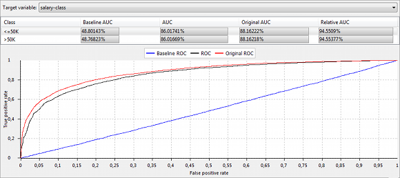
Please note that ARX uses an one-vs-all approach to calculate performance measures for multinomial classifiers.

Data quality models

This section displays measures of data quality obtained for output data using various general-purpose models. In addition, the data types of attributes as well as the fraction of missing values is presented.

The view at the top shows attribute-level quality, i.e. quality estimates that relate to individual quasi-identifiers. The view at the bottom shows data-level quality, i.e. quality estimates for the overall set of quasi-identifiers.

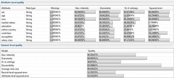
Note that not all quality measures are necessarily supported for all attributes or datasets. If a quality measure could not be evaluated for an attribute, the result is displayed as "N/A" in the upper table. As a consequence, this attribute has also been ignored when calculating data-level quality using the same model.

The following attribute-level quality models are currently implemented:

1. Precision: Measures the generalization intensity of attribute values. For details see: Sweeney, L.: Achieving k-anonymity privacy protection using generalization and suppression. J. Uncertain. Fuzz. Knowl. Sys. 10 (5), p. 571-588 (2002).
2. Granularity: Captures the granularity of data. For details see: Iyengar, V.: Transforming data to satisfy privacy constraints. Proc. Int. Conf. Knowl. Disc. Data Mining, p. 279-288 (2002).
3. Non-Uniform Entropy: Quantifies differences in the distributions of attribute values. For details see: Prasser, F., Bild, R., Kuhn, K.A.: A Generic Method for Assessing the Quality of De-Identified Health Data. Proc. Med. Inf. Europe (2016). and De Waal, A., Willenborg, L.: Information loss through global recoding and local suppression. Netherlands Off. Stat., vol. 14, p. 17-20 (1999).
4. Squared error: Interprets values as numbers and captures the sum of squared errors in groups of indistinguishable records. For details see: Soria-Comas, J., et al.: T-closeness through microaggregation: Strict privacy with enhanced utility preservation. IEEE Trans. Knowl. Data Eng., 27(11), p. 3098-3110 (2015).

In addition, the following dataset-level quality models are available:

1. Average class size: Measures the average size of groups of indistinguishable records. For details see: LeFevre, K., DeWitt, D., Ramakrishnan, R.: Mondrian multidimensional k-anonymity. Proc. Int. Conf. Data Engineering (2006).
2. Discernibility: Measures the size of groups of indistinguishable records and introduces a penalty for records which have been completely suppressed. For details see: Bayardo, R., Agrawal, R.: Data privacy through optimal k-anonymization. Proc. Int. Conf. Data Engineering, p. 217-228 (2005).
3. Ambiguity: Captures the ambiguity of records. For details see: Goldberger, Tassa.: Efficient Anonymizations with Enhanced Utility. Trans. Data. Priv.
4. Record-level squared error: Interprets records as vectors and captures the sum of squared errors in groups of indistinguishable records. For details see: D. Sanchez, S. Martinez, and J. Domingo-Ferrer.: Comment on unique in the shopping mall: On the reidentifiability of credit card metadata. Science, 351(6279):1274-1274, 2016.

Local recoding

This section of ARX's utility analysis perspective enables users to perform local transformation (involving multiple transformation methods, e.g. generalization and aggregation) to further enhance the quality of output data obtained via a primary anonymization procedure. It is recommended to perform primary anonymization using a suppression limit of 100% and a configuration which favors suppression over other types of data transformation. The latter can be configured by moving the slider in the "coding model" section of the configuration perspective to the leftmost position. Then, local recoding can be performed in this perspective with various methods. It is recommended to use the default configuration (slider moved almost to the left, method: fixpoint-adaptive with parameter 0.05).

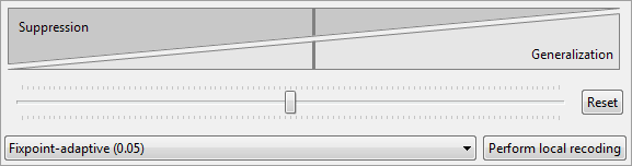
ARX will perform local recoding by recursively executing a global transformation algorithm on records that have been suppressed in the previous iteration. With this method, a significant improvement in data quality can be achieved, even in comparison to other local transformation algorithms. Moreover, the method supports a wide variety of privacy models, including models for protecting data from attribute disclosure.

Please note that local transformation is supported more explicitly since version 3.7.0 of ARX and that this view is typically not needed anymore.