Help: Lattice

Visualization of the solution space (area 1)

In the center of the screen, the view displays a subset of the current solution space. The space may be visualized in different ways. Firstly, it can be displayed as a Hasse diagram.

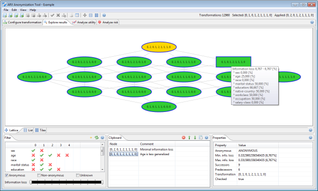
Here, each node represents a transformation and is identified by the generalization levels that it defines for the quasi-identifiers in the input dataset. Transformations are characterized by three different background colors:

1. Green denotes that the transformation results in an anonymous dataset
2. Red denotes that the transformation does not result in an anonymous dataset
3. Orange denotes that the transformation is the global optimum

Transformations that have been checked explicitly be the tool are marked with a thick blue border. Dragging the mouse while holding the left button will move the current section of the solution space. Dragging the mouse while holding the right button will zoom in and out of the current view. Hovering the mouse over a transformation will display a tooltip with basic information about the transformation. Clicking a transformation with the left button will select it, while clicking a transformation with the right button will bring up a context menu. Here, transformations can either be applied to the current input dataset or added to the clipboard. Secondly, the solution space may be displayed as a list.

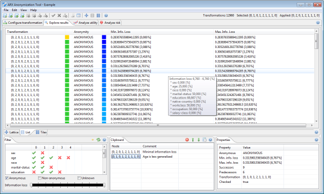
Here, each transformation is represented by one row. Rows are sorted by information loss. Data utility and the anonymity property are highlighted graphically. Thirdly, the solution space may be displayed as a set of tiles.

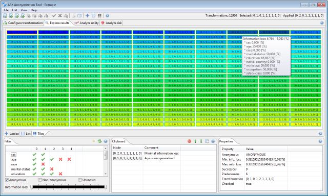
This view is very similar to the list described in the previous paragraph. The color and border of an element encodes information about the anonymity property, while the background color represents data utility. Elements are also ordered by their utility.